THU-BDC2026 Experiment Log - Those Optimizations That Made the Results Worse and Worse
Conclusion First
What is most worth recording about THU-BDC2026 is not some return that looks beautiful once, but those experiments that pulled the model back from “looks effective” to “actually verifiable”.
This is my experiment log. It does not seek to package the project as smooth sailing; instead, it specifically writes down several optimizations that made the results worse and worse, because the experience that can truly remain in a competition is often hidden in these failures.
| Time | Experiment | Result | My Judgment |
|---|---|---|---|
| 2026-05-31 | Single-period backtest | Latest dataset model, single week +5.9533% | Very bright, but the period is too short; can only be a clue |
| 2026-06-04 | Fixing data leakage | Sharpe dropped from 2.30 to -0.49 | Ugly, but finally honest |
| 2026-06-05 | Removing volatility features | Features 289 -> 227, Sharpe back to 0.40 | Subtraction works |
| 2026-06-06 | Adding money flow factors | Sharpe 0.70, cumulative return 12.33% | The most decent version so far |
| 2026-06-06 | Top-80 feature selection | Training 57% faster, return dropped to -7.47% | Fast does not equal good |
| 2026-06-07 | Industry coverage fix | Coverage 4.7% -> 100%, Sharpe fell to 0.18 | Data completeness does not mean the model can use it |
Why Write It as a Log
At the beginning, this project could easily get people carried away: complex models, rich metrics, and some backtest results that looked very strong.
But what quantitative projects fear most is “abnormally pretty”. As long as there is a little future information in the training set split, label construction, or feature window, the model will become stronger as if it suddenly got it. The problem is that this kind of strength is not real strength; it just saw the answer in advance.
So the focus of this article is not “how powerful a model I built”, but recording how I squeezed out the fluff step by step:
- First, acknowledge that single-period results cannot be conclusions;
- Then fix the time isolation between training and prediction;
- Next, delete features that may depend on leakage;
- Finally, see which factors can still retain real gains.
Early Single-Period Backtest: Very Bright, but Not to Be Trusted Too Much
There is an early backtest report in the archive; it only tested the 5 trading days from 2026-03-09 to 2026-03-13.
At the time, the results looked very good:
| Model | Single-period return |
|---|---|
| Original dataset model | -0.7367% |
| Latest dataset model | 5.9533% |
| Equal-weight benchmark | 1.3114% |
If you only look at this table, it is easy to feel that the direction is already right. But 5 trading days is too short, and luck plays a big role. It is more like a hint: “There may be something here, worth investigating further,” but it cannot prove that the model is stably effective.
Looking back later, the greatest value of this stage was not the return, but the reminder that I had to lengthen the validation period and make the backtesting process stricter.
Fixing Data Leakage: The Most Painful, but the Most Worthwhile
What truly changed the direction of the project was fixing data leakage.
The original backtest only ensured that training sample dates were earlier than the backtest date, but the labels used the opening prices of the next 5 days. That is, for training samples close to the backtest date, although the dates were in the past, the labels might already extend into the future window.
This type of leakage is very hidden. The code looks fine, and the results look very good, but in essence the model has already peeked at the answer.
After the fix, the results immediately became ugly:
1 | Sharpe: -0.49 |
This step was very discouraging, but it was the most important step in the entire experiment line. Because from here on, the later results are worth discussing.
Subtraction: Cutting Volatility Features
After fixing the leakage, I began to suspect a batch of volatility-related features.
For example:
boll_widthatr_pctvol_20d- Aggregate features and cross-sectional rank features derived from these indicators
They had very high importance in the old version, but the old version itself had leakage. So I was not sure whether they were truly effective or just helped the model memorize shortcuts in the wrong validation.
So I ran a deletion experiment:
1 | Feature dimension: 289 -> 227 |
This time the results actually got better. The reminder it gave me was very direct: more features are not safer. Especially in financial data, some features seem to have a lot of information, but in fact they just amplify noise and wrong validation together.
Money Flow: One of the Few Things That Truly Brought Gains
Later I added Tushare money-flow-related factors, mainly including three categories:
- Main-force net inflow rate;
- Small-order net inflow rate;
- Super-large-order share.
This version is a relatively decent one in the current experiment log:
1 | Sharpe: 0.70 |
More importantly, 主力净流入率_ma20_cs_rank entered the top 20 feature importances.
This made me feel that capital behavior signals may be more valuable than simply stacking price patterns. Price patterns easily overfit; money flow at least provided another type of information in this window.
Three Failed Optimizations
Top-80 Feature Selection
I used data before 2023 to select the 80 most important features, wanting to reduce noise and speed up training.
Training speed did indeed become faster:
1 | Training time: 116 minutes -> 50 minutes |
But the results got worse:
1 | Cumulative return: +12.33% -> -7.47% |
This shows that importance in a historical window does not necessarily transfer to the future. Financial data is not a static dataset; once the market regime changes, the features that were most important in the past may instead hold it back.
Three-Class Labels
I also tried roughly dividing stocks into three tiers:
- Top 30%;
- Middle 40%;
- Bottom 30%.
The intention was to make the model focus more on the “buy zone” and the “risk-avoidance zone”, but the actual effect was very poor, and the Sharpe fell to -1.08.
The reason is probably that a ranking task cannot be cut too coarsely. Although 10-bin labels are a bit more complex, they retain more relative order information and are more suitable for selecting the Top 5 from 300 stocks every day.
Industry Coverage Fix
There was also a very counterintuitive failure: the industry coverage fix.
Originally industry coverage was only 4.7%, which was certainly unreasonable, so I filled the industry information to 100%. From the perspective of data completeness, this step was absolutely correct.
But model performance dropped from a Sharpe of 0.70 to 0.18, and sector_id became the most important feature.
This shows that the model may not have “learned the industry” but rather “trusted the industry too much”. Industry information needs finer constraints, such as downweighting, regularization, and grouped validation; it cannot just be stuffed in all at once.
Rules Left in the End
After this round of experiments, I left myself a few rules:
- Single-period results can only be clues, not conclusions.
- The first step of backtesting is always to check for data leakage.
- Feature importance should be viewed by time period; one historical window cannot be treated as truth.
- Subtraction is not shameful; being able to remove noise is also a skill.
- More complete data also needs to be used correctly by the model.
- All changes that “look reasonable” must ultimately let the backtest speak.
What to Do Next
If I continue advancing this project, I will prioritize three things:
- Lengthen the rolling backtest period and stop being led by single-week returns;
- Perform grouped validation on strongly structural features such as industry, market cap, and liquidity;
- Keep LightGBM LambdaRank as the main line, and treat deep models as auxiliary experiments rather than the main battlefield.
This record does not constitute any investment advice. It is more like a competition experiment memo: break open the good-looking results, keep the ugly-looking results, and only what remains in the end may be real experience.